Introduction

Purpose

cuNLS is a CUDA/C++ library for solving nonlinear least-squares problems on the GPU. It is designed around batched factor evaluation, sparse Jacobian assembly, and sparse linear solvers tailored for large scale minimization problems.

cuNLS also provides pycunls, a Python package that exposes the full C++ API through CuPy-based GPU arrays (see pycunls Installation). For advanced extensibility, pycunls integrates with NVIDIA Warp to let users author custom factor and state kernels in Python (see Python Tutorial).

Nonlinear least-squares problems

At a high level, cuNLS solves optimization problems of the form:

\[x^* = \arg\min_x \sum_i \rho_i\left(\left\|f_i(x)\right\|^2_{\Sigma_i}\right)\]

where:

• \(x\) is the optimization variable (often living on a manifold),

• \(f_i(x)\) are residual/error functions,

• \(\rho_i(\cdot)\) are optional robust loss functions,

• \(\left\|v\right\|^2_{\Sigma} = v^T \Sigma^{-1} v\) is the Mahalanobis norm.

Using a square-root information matrix \(R_i\) such that \(\Sigma_i^{-1} = R_i^T R_i\), each term can be rewritten as:

\[\left\|f_i(x)\right\|^2_{\Sigma_i} = \left\|R_i f_i(x)\right\|^2\]

This is exactly why cuNLS has a dedicated InformationFactorBatch: it applies this whitening step directly to residuals and Jacobians. In C++, the template InformationFactorBatch<T> inherits T::sized_layout (the same SizedFactorBatch as the inner batch). WeightedFactorBatch<T> does the same for scalar weighting.

To solve the nonlinear problem, cuNLS linearizes around the current estimate \(x_0\):

\[f_i(x_0 + \Delta x) \approx f_i(x_0) + J_i \Delta x\]

Stacks all blocks into a global Jacobian \(J\) and vector \(b\), then solves a sparse linearized system (Gauss-Newton / Levenberg-Marquardt):

\[\Delta x^* = \arg\min_{\Delta x} \left\|J\Delta x + b\right\|^2\]

with normal equations:

\[J^T J \Delta x^* = -J^T b\]

and updates:

\[x^* = x_0 \oplus \Delta x^*\]

where \(\oplus\) is the manifold plus operation implemented by state batches (for Euclidean states, this reduces to simple addition).

Factor Graphs

A common way to set up nonlinear least-squares problems is to create a factor graph: a graph where nodes represent variables and edges represent constraints between them.

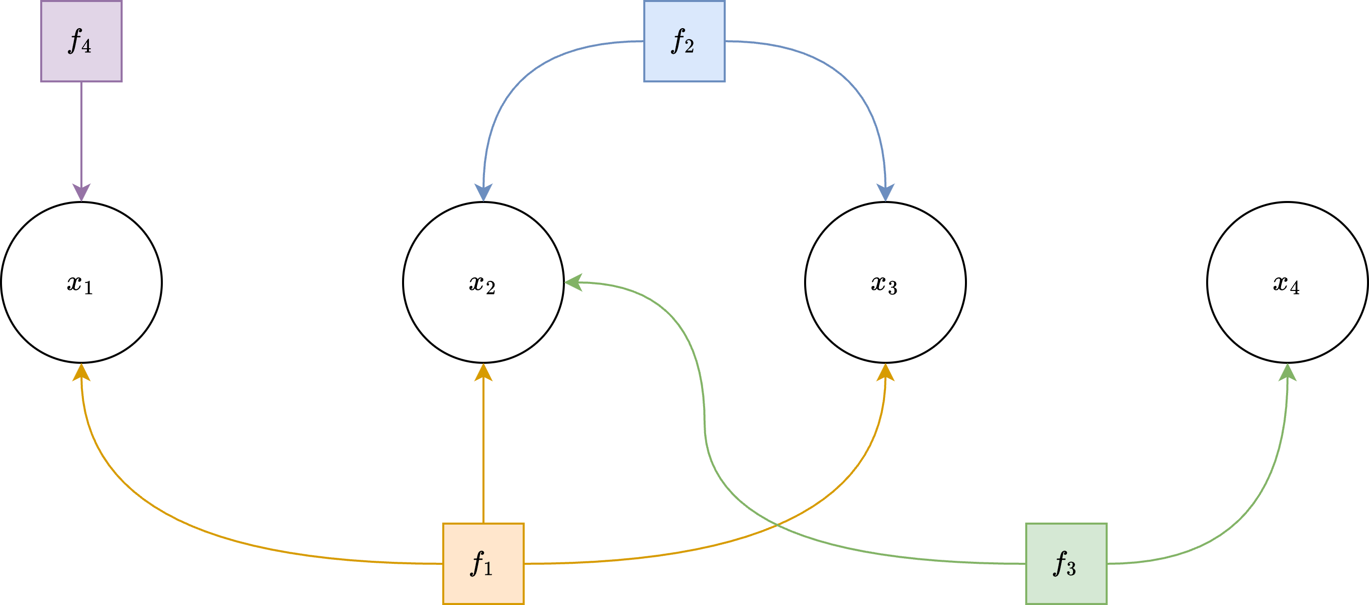
Example factor-graph structure used to represent sparse nonlinear least-squares problems.

The constraints between variables are called factors, which are nonlinear functions representing mean error. Each factor is also associated with a covariance matrix. Together the mean and the covariance represent multivariate normal distribution for a given factor.

This way factor graph is a probabilistic graphical model, which represents a joint probability distribution of all factors

\[p(x) \propto \prod_i p_i(x_i)\]

and the MAP estimate is:

\[x^* = \arg\max_x p(x)\]

For Gaussian-like factors:

\[p_i(x_i) \propto \exp\left(-\frac{1}{2}\left\|f_i(x_i)\right\|^2_{\Sigma_i}\right)\]

maximizing the posterior is equivalent to minimizing the sum of squared (and optionally robustified) residuals.

cuNLS allows setting up variables and factors in batches for higher GPU utilization. A FactorBatch is a collection of same type factors that are connected to a list of StateBatch objects — collections of same type variables. The Problem is a collection of FactorBatch objects and connected StateBatch objects, that together form the Factor Graph.

Core concepts

• State batches store optimization variables on manifolds (for example, SE3StateBatch for rigid transforms, VectorStateBatch<Dim> for Euclidean vectors).

• Factor batches compute residuals and Jacobians in parallel for many observations.

• Problems connect factors to states via device pointers.

• Minimizers (GaussNewtonMinimizer, LevenbergMarquardtMinimizer) solve for state updates.

• Loss functions robustify residuals to reduce outlier influence.

High-level solve flow

1. Allocate state data on the GPU.

2. Wrap state memory in one or more StateBatch objects.

3. Build one or more FactorBatch objects from observations.

4. Add state batches and factor batches to a Problem.

5. Run a minimizer and inspect MinimizerSummary.

Supported optimization patterns

• Pose graph optimization with between factors.

• Bundle-adjustment style reprojection optimization.

• ICP-like alignment (point-to-point / point-to-plane factors).

• Custom user-defined factors through FactorBatch / SizedFactorBatch.

See Tutorial for complete C++ working pipelines, Python Tutorial for Python examples, and API Reference for class-level API details.